SAP Data Warehouse Cloud, it’s time to talk about it…


I’ll admit I haven’t posted too much about SAP Data Warehouse Cloud (DWC) over the last few years. In part it was due to being heads down working on projects, managing a BI practice, and lacking time to see what makes it work. However, I have had just enough time over the last few months to really dig into the platform and see what it can do, and I am quite excited about what I learned. Frankly, the experience was much like the first time I did the same with SAP HANA some 10 years ago. As a result, I plan to ramp up blogging again and share my thoughts on the platform. To start things off, l will list out a few items I think will really resonate with clients who are seeking a quick overview of what makes DWC unique and exciting. Below are a few of my thoughts on DWC.

Replication of data

I really like how simple DWC makes provisioning and replicating HANA DB tables, S4/HANA CDS Views and ECC ODP extractors into the platform. The architecture and user interfaces are very well put together, simple to setup and use. Replication is a critical component or requirement in my modern agile EDW methodology. While this was achievable with SLT and a HANA database, the architecture was a bit much to setup and manage. With DWC, only two lightweight agents (DP Agent and SAP cloud connector) are required to replicate data securely into DWC. This light architecture makes managing the architecture much simpler. Couple that with DWC being a SaaS platform, organizations will be able to spend more time developing and innovating and less time maintaining and upgrading.

Focus on End Users and IT developers

DWC’s UI is well suited to support advanced IT developers and self-service business users. The data builder, business builder, focus on meta data and space management work well together in producing a shared environment where both IT resources and business users can model and blend data. I can really see how this type of experience can bring about a simpler data governance process for organizations.

Open Connectivity

DWC offers a large array of support for both SAP and non-SAP source systems.  Data can be provisioned from many modern on-premises databases and popular cloud data platforms. With a HANA ODBC client, many data platforms and BI Tools can easily consume data from DWC. Combine this with the fact that you can easily replicate and model data from SAP systems, you will find it an ideal platform to expose SAP data and models to other platforms and tools. 

The BW Bridge

The BW Bridge is a fascinating add-on to DWC. It offers a literal “Bridge” where organizations can leverage their past investments in SAP BW by moving Extractor code, aDSO, transformations, BW master data and composite providers to the cloud. Not only can you move them to DWC but we can continue to load data from SAP systems as if it were a normal BW4/HANA system. Based on SAP’s road map, many BW Queries will soon be supported in the platform. The BW bridge is not a full implementation of BW4/HANA in the cloud. You can think of it as a partial implementation where supported BW models can be used as data sources in DWC. Once exposed to DWC, you will be required to further model them into DWC compliant models. However, if an organization has value in the current BW models and queries, the BW bridge is a quick and easy way to get them started with DWC. The BW Bridge also has standard BW4/HANA content that can be deployed for those seeking a quick way to get a “greenfield” implementation of DWC up and running.

Model with SQL

DWC offers the ability to model data using SQL Statements and Scripts. While the graphical modeling tools are great to have, being able to model in SQL and even port SQL code over from other platforms, make DWC easier to adopt and more flexible for BI and EDW developers well versed in SQL coding. This might seam like an odd feature to call out, but legacy solutions like SAP BW were centered more around ABAP development and GUI wizards for data modeling. SQL is a more universal data modeling language which makes it easier for a general BI developer or advanced power user to work in DWC.

Flexible Storage Tiers

When source tables and CDS Views are initially imported, no data is moved to DWC. While you can query this virtual table entity within DWC, it is initially federated from the source in real-time. You can later choose to batch load the data or replicate the table / CDS View into disk bound storage within DWC to improve query performance. Furthermore, you can choose to have that same data bound to in-memory storage with the toggle of a button. This flexibility allows you to define a simple, per table entity, storage tier for data. Organization can even incorporate the SAP HANA Cloud Data Lake into their cloud landscape giving them even more cost-effective storage options for structured and unstructured data.

HDI Container

DWC supports the deployment of a HANA HDI container. Within this container and using BTP developments tools, organizations can model data using for example SAP HANA XSA Calculation Views. Organizations could even import existing SAP HANA XSA HDI container content into the platform when migrating from an existing HANA DB environment. This is yet another way organizations could migrate existing content into DWC to rapidly get results.

In the upcoming months, I plan to release more blogs and content on DWC. I look forward to hearing about you experience in the comments below.

The SAP Business Intelligence Roadmap


The SAP Business Intelligence Roadmap: Evolution and Convergence

By Jonathan Haun, Senior Director, BI and Technology

Many of our clients want to know how best to navigate SAP’s business intelligence roadmap but the SAP reporting and analytics ecosystem has a complex history that continues to evolve. Enowa’s Senior Director, Jonathan Haun, an accomplished author and thought leader in this space, offers some insights.

How We Got Here

Since SAP’s acquisition of BusinessObjects in 2007, the SAP roadmap for Business Intelligence (BI) has evolved dramatically and quickly from its legacy solution, SAP Business Warehouse. When SAP introduced SAP HANA, a revolutionary data platform, in 2010, it represented the next fork in the company’s BI roadmap. Many organizations chose to leverage SAP HANA by moving their instances of SAP BW to SAP BW on HANA. Others used SAP HANA directly using batch ETL or real-time replication with HANA modeling. Because SAP BusinessObjects is capable of interfacing with both SAP BW on HANA and Native SAP HANA, organizations could choose between either BI platform solution. SAP HANA continues to be the data storage backbone of most SAP BI solutions, both on-premise and in the cloud. SAP BW on HANA has further evolved into SAP BW/4HANA and its most recent version has significantly simplified data management, lifecycle management, transformations, and data lineage.  

Early Self-Service Visualization Tools

As SAP continued down the road to self-service and visualization, many more forks appeared in the roadmap. SAP BusinessObjects included a powerful ad-hoc reporting tool named Web Intelligence (WebI). While WebI is an excellent tool, end-users often require training to use it. In 2012, SAP introduced the self-service BI tool SAP Visual Intelligence (later renaming it SAP BusinessObjects Lumira 1.0). In 2013, SAP also introduced a developer focused dashboard tool, SAP BusinessObjects Design Studio. Design Studio could produce niche data visualizations and web-based BI applications but required a skilled programmer. To address the demand for easier self-service tools, SAP introduced SAP Lumira 2.0 in 2017, which combined SAP Lumira 1.0 for self-service and SAP BusinessObjects Design Studio for professional developers. SAP Lumira 2.0 made it possible for end users to create visualizations and then pass their work on to a professional developer for niche customizations.

SAP SAC: Cloud Analytics

In 2018, SAP introduced SAP Analytics Cloud (SAC), another significant fork in the BI roadmap. This platform and its capabilities represent the current roadmap for SAP Business Intelligence visualizations, dashboards, planning, predictive analytics, and advanced analytics capabilities. However, the solution does not always address some important BI needs—particularly around data security, enterprise reporting, and report distribution. To that end, SAP will introduce SAP BusinessObjects 4.3 this year, bringing together SAC’s capabilities combined with SAP BusinessObjects Enterprise. A stated goal of SAP BusinessObjects 4.3 is to increase the integration capabilities between SAC and SAP BusinessObjects Enterprise. With that said, SAP issues updates to SAC often and these updates continue to address my concerns more often then not.

SAP Data Warehouse Cloud

Another significant fork in the road for SAP BI was the introduction of SAP Data Warehouse Cloud in late 2019. SAP Data Warehouse Cloud (DWC) is another SAP HANA-based SaaS offering that provides data storage, data transformation, ELT, ETL, data semantics, data cataloging, and data modeling all within a scalable cloud platform. It doesn’t necessarily replace SAP BW nor HANA, but there is a significant overlap of functionality between SAP DWC and on-prem solutions like SAP BW and Native SAP HANA. With that said, their is no easy migration path from SAP BW to DWC and getting to this platform will take some manual redevelopment. Their are options to migrate HANA XSA (container based) content to DWC but it too requires some manual intervention and be ready for a complex setup. The SAP DWC BW Bridge is also available which would allow an organization to migrate about 80% of their SAP BW4/HANA content to DWC. The remaining 20% would then need to be modeled using DWC modeling techniques.

Core Data Services for Operational Reporting

S/4HANA has also disrupted the BI strategy, creating yet another fork in the road for many organizations, with the introduction of Core Data Services (CDS). CDS allows organization to create metadata-rich data models for operational reporting, using a SQL-like language that makes it easier to model data. CDS also works with the Embedded SAP BW, a solution native to SAP NetWeaver starting with version 7.0 and beyond, to provide enhanced metadata and reporting capabilities. Most organizations will find this combination a viable option to support operational BI reporting within the S/4HANA landscape. This same architecture also supports embedded analytics common to many SAP-provided Fiori GUI interfaces. SAP also provide a large library of prebuilt SAC content that can be connected to S/4HANA CDS prebuilt and custom models.

What’s the Best SAP BI Roadmap for You?

SAP has rapidly evolved their BI platforms, capabilities, and BI tools over the last 20 years and at a pace that most customers cannot match. As a result, many customers find themselves leveraging one of SAP’s many BI solutions, which automatically sends them down one of the many forks in the SAP BI roadmap. To further complicate matters, not every solution stack provides the same functionality and organizations may risk failed adoptions if they try to move business users to a solution that does not quickly solve their problems.

While every organization is different, some best practices still apply. Organizations should catalog their current landscape, tools, and data lineages with the goal of assessing their current state and identifying their data pipelines. IT should also conduct workshops with business users and data owners to better understand their data pipelines, KPIs, metrics, needs, and identify any gaps or issues. That will give IT a better understanding of how best to align business needs with SAP’s current roadmap. It’s also important to remember that your data management strategy is likely the most important component for successful self-service BI enablement. In my experience, most organizations place too much emphasis on the end user reporting tools and fail to properly govern the data pipelines that feed their KPIs and metrics.

Final Thoughts

SAP, like many other providers, is moving its tools and solutions to the cloud. But bear in mind that this doesn’t mean that legacy tools like SAP BW, native SAP HANA or SAP BusinessObjects should be abandoned, especially if your organization has invested in content that will not easily be migrated to SAP’s SaaS offerings without significant redevelopment. Therefore, I suspect that most organizations will embrace a strategy where their on-premise architectures are modernized, consolidated, and streamlined before content is moved into SAP’s SaaS platforms.

About the Author

Jonathan has been an IT leader for over 20 years, helping clients implement successful business intelligence and data management solutions. He has authored, or co-authored, several books about SAP HANA and routinely speaks at SAP conferences on BI, HANA and other security topics. Jonathan is a Senior Director at Protiviti, responsible for managing and delivering Protiviti’s SAP and non-SAP BI initiatives. He also helps clients with their SAP HANA implementations, SAP IaaS cloud deployments, and SAP HANA Security models.

Passing Multiple Input Parameter Values in a Calculation View to a Table Function Filter


Developers often find it useful to utilize a table function (.hdbtablefunction) as the base projection within their calculation views. When this option became available, it effectively replaced the need to create script-based calculation views. Table Functions offer advanced SQLScript and SQL coding that can allow you to greatly enhance the performance of query execution with the use of variables for filtering. Calculation Views offer variables and input parameters. Variables can easily support multiple values for filtering, but the filter logic might not be pushed to the lowest levels of the query execution depending on the complexity of the model and table function SQL. Input parameters can be created in the calculation view and then mapped to the input variables on a table function. For single value input parameter values, this is very straight forward. You effectively define an input parameter in the calculation view and an input variable in the table function. Map the calculation view input parameter to the table function input variable. Within the table function, you define a filter in the WHERE clause setting some column equal to the input variable.

However, if the HANA calculation view’s input parameter is defined as “multiple value” we run into issues passing the values into the table function’s WHERE clause. Based on my tracing, I can see that the input parameter passes an array of values to the table function as a string. For example, if we have a HANA Calculation View input parameter called IP_PLANT that support multiple values and the user executes the calculation view, configuring two plants (1000,1001) in the input parameter screen, the calculation view would pass the string ‘1000’,’1001’ to the variable in the table function. If the table function WHERE clause has WERKS IN ( :V_PLANT ), you get no data returned. From what I can tell what is actually being executed is WERKS IN ( ‘ ‘1001’,’1000’ ‘). Note the extra single quote around the array which cause the WHERE clause to look for a string lateral value of ‘1001’,’1000’. Because these additional single quotes are applied at run-time, there is no way that I could find to remove them before the SQL was compiled.

With that said, I was able to find a workaround to this problem using some of the advanced capabilities of the table function script. Without using the WHERE clause of the table function SQL, there is a way to dynamically apply a filter to a table, table variable or view using a function called APPLY_FILTER(). This function accepts two inputs. APPLY_FILTER( <Table>, <Filter String>) and this function is defined the SQL before the RETURNS statement and compiled with the SQL. Below, I will walk you through the complete setup.

  1. Define a calculation view with two input parameters that is based on a table function.

2. Input Parameter (For this example) is defined as follows.

  • Multiple Entries
  • Is Mandatory
  • Default Value of * – We will use this in the filter string to return all values when * is selected.
  • List of Values from table

3. We will map the input parameter to the table function input variable

4. We define the table function script as follows:

FUNCTION "JHAUN"."xxx_sandbox.poc3::TF_JH_TEST" ( V_MATERIAL_GROUP NVARCHAR(1000), V_MATERIAL_TYPE NVARCHAR(1000) ) 
	RETURNS TABLE ( 
	MATERIAL NVARCHAR(18),
    	BASE_UOM NVARCHAR(3),
    	MATERIAL_GROUP NVARCHAR(9),
    	MATERIAL_TYPE NVARCHAR(4),
    	WEIGHT_UOM NVARCHAR(2),
    	NET_WEIGHT Decimal(17,3),
    	PRODUCT_HIERARCHY NVARCHAR(18),
    	MATERIAL_STATUS NVARCHAR(5),
    	FILTER_STRING NVARCHAR(10000)
 					)
	LANGUAGE SQLSCRIPT
	SQL SECURITY DEFINER AS
BEGIN


DECLARE MY_FILTER varchar(10000) := '(''*'' in (' || :V_MATERIAL_GROUP || ') or MATKL in (' || :V_MATERIAL_GROUP || ')) and ( ''*'' in (' || :V_MATERIAL_TYPE || ') or MTART in (' || :V_MATERIAL_TYPE || '))';

BWTABLE = APPLY_FILTER( SAPHANADB."/BIC/AY_MATRIAL2", :MY_FILTER );

RETURN 

SELECT
	MATNR AS MATERIAL,
	MEINS AS BASE_UOM,
	CASe WHEN MATKL = '' THEN '00' ELSE MATKL END  AS MATERIAL_GROUP,
	MTART AS MATERIAL_TYPE,
	'LB' AS WEIGHT_UOM,
	NTGEW AS NET_WEIGHT,
	PRDHA AS PRODUCT_HIERARCHY,
	MSTAE AS MATERIAL_STATUS,
	'MATKL in (' || :V_MATERIAL_GROUP || ') and MTART in (' || :V_MATERIAL_TYPE || ')' AS FILTER_STRING
	
FROM :BWTABLE


UNION ALL

SELECT
	null AS MATERIAL,
	null AS BASE_UOM,
	null AS MATERIAL_GROUP,
	null AS MATERIAL_TYPE,
	null AS WEIGHT_UOM,
	null AS NET_WEIGHT,
	null AS PRODUCT_HIERARCHY,
	null AS MATERIAL_STATUS,
	'MATKL in (' || :V_MATERIAL_GROUP || ') and MTART in (' || :V_MATERIAL_TYPE || ')' AS FILTER_STRING
	
FROM DUMMY;

END;

4. There are several items in this example table function that are included for troubleshooting purposes. However, the core of the solution centers around the “DECLARE MY_FILTER varchar(10000)” and the “BWTABLE = APPLY_FILTER( SAPHANADB.”/BIC/AY_MATRIAL2″, :MY_FILTER )” sections before the RETURNS clause.

               DECLARE MY_FILTER is a variable we use to craft the filter clause string from the two input variables.  Once compiled, the string would be (for example) (‘*’ in (‘T01,’T02’) or MATKL in (‘T01,’T02’)) and ( ‘*’ in (‘ZPCF’,’TERT’) or MTART in (‘ZPCF’,’TERT’)) . This is very similar to how SQL based Analytics Privileges work in situations where we directly define the filter clause. The difference here is that we dynamically craft the string based on what calculation view input parameter are passed.

               BWTABLE = APPLY_FILTER section is used to set a table variable equal to the APPLY_FILTER function. In the function we specify the table where we want to apply the filter and also the filter condition string.

               In the RETURNS SQL, we SELECT FROM the table variable :BWTABLE and not the actual table in the database. For added value in troubleshooting, I added a string constant to output an example of the filter conditions and a UNION from dummy to always return an example of the filter conditions even if no matching data was found. These were only added for troubleshooting purposes and would not be needed in a production grade table function.

This is just a basic example but it demonstrates how you can pass multiple values from a calculation view into a filter condition in a table function. Their are other methods documented that can be found on the internet. For example, you can use another table function to convert the string array into a results table. You can then use this table function and it’s results table in a WHERE clause sub-select. However, based on my plan visualization testing, the APPLY_FILTER method out performs the WHERE clause sub-select method rather significantly. The APPLY_FILTER actual gets applied at the lowest levels when accessing the referenced table. The WHERE clause sub-select method seams not apply the record filtering until near the end of the query execution. Hopefully this will help you get started on creating your own version.

Using SAP Analytics Cloud (SAC) to analyze COVID-19 Data


The following is a recording of a presentation where I demonstrate a SAC dashboard I created to analyze COVID-19 data.

  • No matter what the data indicates or what I say, listen and adhere to all warning and suggestions from the WHO and CDC. This also includes all warning and suggestions from your local, state or federal government.
  • We are analyzing data. However, please remember that this disease impacts real people. Any life impacted or lost should not be marginalized and nothing I present is attempting to do that. I am simply presenting the data and providing analysis.

Video Presentation

Data

COVID-19 Data

SAC Export

FPA_EXPORT_T_2F_SACCOVID19

Interesting Articles:

https://www.statnews.com/2020/03/17/a-fiasco-in-the-making-as-the-coronavirus-pandemic-takes-hold-we-are-making-decisions-without-reliable-data/

SAP BusinessObjects 4.2 SP6+ ONE Installer


One major improvement in SAP BusinessObjects, starting with 4.2 SP6 Patch 100, is the addition of the “ONE Installer”. The “ONE Installer” allows you to update your installation in a single step. In the past, when updating from one support pack (SP) to the next, we had to first install the SP update then apply the latest patch update. This was a two step process that was very time consuming for most administrators. The “ONE Installer” avoids this by allowing us to update directly to a combined SP and Patch version in a single step.

So how does this work you might ask? The process is very simply. You must look for a special update package in the SAP software download site. Under the installations and upgrades section of the download site, you will find a dedicated section called SBOP BI PLAT ONE INST 4.2. As of 7/24/2019 you will find One Installer packages for several items up to support pack 6 patch 0 and also support pack 4 patch 6. Its a little confusing as to why this section only contains SP6 P0 and SP4 P6?

SAPONEInstaller

However, under the SUPPORT PACKAGES & PATCHES section we can find more ONE installer packages for the most recent Support Package and Patch versions. Look for any package name that ends in ” – ONE” once you drill down into a particular section. In some cases, larger packages are split into multiple RAR archives. In such cases the package name will end in” – ONE 1/2″ or ” – ONE 2/2″

SAPONEInstallerUpdates

From what I can tell, there are ONE installer packages for the core SBOP server components, client tools, crystal reports, the explorer plugin, Crystal Reports 2016, Information Platform Services (IPS), Crystal Server 2016, Crystal Reports for Enterprise, Integration for SharePoint,  Live Office and even the Edge Edition. I did not find a ONE installer for Lumira Server or Discovery or the Analysis for Office plugin.

But there is more to the “One Installer” than just simplified updates. ONE Installer supports “Full Installs” as well as updates. For a net new system, we can directly install the latest SP and patch in a single step. For existing systems, we can update a Support Package/Patch to any Support Package/Patch level in a single step.

I recently use the latest 4.2 SP7 Patch 400 ONE installer to update a 4.2 SP6 Patch 300 single node instance. The process was very easy and saved me a lot of time. For reference the process took about 3 hours end-to-end (excluding download time). In the past, I would invest almost double that time on a single server node applying first the SP then the patch. Great addition that will save admins lots of time.

The advantages should be obvious but here are a few that SAP lists for reference:

  • New customers can update directly to the latest Patch level of the latest available Support Package + Patch in a single step.
  • Existing customers can eliminate the step of updating the server landscape to a Support Pack (SP) level before patching.
  • Adding New Nodes becomes a simple process as you can directly run the “SP+ Patch” ONE installer in expanded mode. [no need to run SP then Patch].
  • Save approximately 50% of the install time since two steps of patching are reduced to one step.
  • Reduced production downtime during updates, for end users.
  • Perform validation and testing only once after updating to the required Support Package or Patch.
  • Better maintenance experience for BI Platform administrators.
  • There is no need to request for a combined installer explicitly starting SP06.

I would add that combining this with the phase wise installation option, one where we can “pre-deploy” new update content before down-time begins, will greatly reduce downtime in all SAP BusinessObjects Enterprise Environments.

For more information, see SAP KBA 2671301

My advice to help you reduce your costs when implementing SAP HANA based solutions.


The path to SAP HANA for most SAP customers is now clear. At some point soon, all SAP clients will have to implement HANA if they want to use SAP’s latest and greatest software versions. However, moving to SAP HANA can be very costly if you are not familiar with all your purchasing options. In terms of purchasing the SAP HANA platform, there are three major categories of cost. Software, Hardware and Implementation services. In this blog I will discuss some of the options I have seen customers choose over the last 6 years and include some of my own opinions. Hopefully this will help you save the most money when implementing SAP HANA.

Software licensing

Software licensing cost can be a very significant portion of the initial SAP HANA implementation cost. While each situation is unique and individual contracts can differ, SAP does seem to offer a lot of different ways to purchase HANA.

  • One way is based on the total memory allocation. Such licenses are often offered in increments of 64GB of total RAM allocation and can cost anywhere from $20,000 – $160,000 USD for each 64 GB increment. With this type of license, there are three subcategories of available additions. Standard, Enterprise and Express addition. Note that the SAP HANA Express software is free of charge if you are willing to register with SAP. Each edition has a price point and list of usable functionalities. Overall, this type of “full use” license is desired by organizations that want to use the SAP HANA platform directly without any limitations. For example, it is often used where SAP HANA is the data warehouse or central data hub for reporting and visualization.
  • As an alternative to the “full use” versions, I would also ask your SAP Sales Representative for limited runtime licenses to support your SAP Application servers running on an SAP HANA Database. In some cases, the license cost for SAP HANA can be very competitive compared to the full use license and compared to what you might be paying today for Oracle, MS SQL, DB2 or other SAP supported OEM databases. Such licenses do have restrictions in how you access and use SAP HANA, but they do allow you to get SAP HANA at a more affordable software license cost.
  • In addition to SAP licensing, you must also consider paying SUSE or RedHat for operating system support and licensing. Using the SAP distribution is highly recommended because you will need access to their SAP specific update repositories and SAP HANA specific support team. In addition, you might have to purchase Virtualization licensing, OEM software to support HANA hardware and backup software licensing. These costs all add up require that you pay multiple vendors.

For more information check out this blog by Owen Pettiford

Hardware

Example SAP HANA Appliance – Image from https://blogs.saphana.com

Hardware cost can be a significant portion of the overall SAP HANA implementation cost. However, there are several ways to reduce or limit your overall hardware costs. Here are a few ways I have helped clients reduce their costs:

  • Tailored Datacenter Integration (TDI) gives clients and implementors the flexibility to “custom” build an SAP HANA server that leverages existing certified storage, networking or servers already in their landscape. It is an alternative to the appliance model where a hardware vendor builds and delivers a complete system that includes compute, storage and network devices in a prepackaged and pre-certified build. Often these appliances are also delivered with components that the client cannot easily administer with existing staff. In my experience this often leads to an appliance with outdated firmware and software. Such components can also be redundant and underutilized leading to a waist of capital. Take for example, many scaleup systems often require multiple disks to achieve the required IOPS. This leads to large (multiple TBs) of diskspace that will never be fully utilized by SAP HANA. I often see the same issue with network switches and fiber channel switches. Only a few ports are populated to support the SAP HANA cluster, leaving several open but never utilized. Therefore, in many cases, the TDI rules can be leveraged to reduce hardware redundancy, maintenance and overall cost.
  • Entry level systems are another way to reduce overall hardware costs. Such systems are typically based on the intel E5 generation CPU and such CPUs are often significantly cheaper than the Intel E7 alternative. As you can see, SAP has listed multiple vendors platforms as “supported” for SAP HANA workloads. https://www.sap.com/dmc/exp/2014-09-02-hana-hardware/enEN/intel-systems.html. Such systems are not as scalable nor powerful as those certified and running on the Intel E7 CPU, but again they are often much cheaper than the alternative. I have built many of these systems over the years and can personally recommend them for clients that have less than 512 – 756 GB of compressed data within their SAP HANA system. They are also great at running non-productive workloads in SBX, DEV and QAS.
  • Reconditioned hardware is also a way to save a lot of money. HANA systems have been around for over 5 years and we are starting to see a lot of used hardware available in the aftermarket that can run SAP HANA 1.0. You know the old saying, “one man’s trash is another man’s treasure”. To give you some perspective, you can often get a Dell R910 systems with 1 TB or RAM, 4 x E7-4870 10-Core CPU and 7 TB of SATA SSD for around $11,000.00 in the aftermarket. This includes a 6 year NBD parts replacement warranty and 10GB SFP NIC cards. Compared to a shiny new system, costing well over $60,000, this is an amazing alternative. Such systems are great at running non-productive workloads and can also be virtualized under the TDI rules.
  • Running SAP HANA in the cloud IaaS style can also save you some money while converting the cost to a monthly operational expenditure. This is sometimes more attractive when compared to a large initial capital expenditure that can be underutilized or alternatively, might become quickly obsolete. In addition, you can reduce other operating costs by shifting and subsequently reducing hardware energy and maintenance costs to a cloud vendor. In general, the cloud argument is not only about the potential for cost savings, it also offers great flexibility in terms of scalability, high availability and disaster recovery. Hybrid cloud deployments can also be leveraged allowing an organization to move a portion of the landscape to the cloud. With AWS specifically, they offer Reserved Instance Pricing at a discounted rate. For example, you can purchase a 3 year, all up-front convertible SAP HANA x1e.2xlarge instance for just under $15,000.00. This is an outstanding price for companies that only need a 244 GB instance of HANA.

Implementation

Implementation costs are another significant factor for most clients. Implementation costs in this case refer to the cost you pay for a person to install your SAP HANA appliance or TDI landscape.

  • When choosing the appliance model, these costs are often built into the package. I have seen them range anywhere from $10,000 – $40,000 depending on the appliance. In most cases, the services provided here are limited to deploying the appliance with little to no post installation configuration. I would argue that most clients need a lot more knowledge transfer, security setup, backup setup and other key items that are often not included in the appliance model services.
  • You can expect the TDI implementation costs to range from $180 – $275 per hour. The price depends on many factors. For example, those seeking someone with the skills to deploy the computer hardware, shared storage, software and virtualization software can be more expensive than those needing a simple SUSE Linux OS on a single node server. TDI implementation services are often overall more competitive, tailored more to your environment and can include add-ons like training, post implementation support, security setup, backup and DR testing and other practical items. In my experience, clients tend to get more value when using a certified TDI implementer.

If you need further consulting help, do not hesitate to contact me via LinkedIn Jonathan Haun or via Twitter @jdh2n

Multistore Table Partitions in SAP HANA 2.0


hana-2-0-extended-storage

Starting with SAP HANA 2.0 we can now partition a single table between in-memory storage and SAP HANA Extended Storage (AKA.. Dynamic Tiring). This is an excellent feature because it simplifies the management and code required to manage multiple tables and subsequently bridge them together using additional code. Basically, we can establishing archiving within our tables without the need to move the data into separate tables.

Prior to SAP HANA 2.0, we would have to create two identical tables. One would be provisioned in-memory and the other in extended storage. We then had to create catalog views or SAP HANA Information Views to logically merge the tables together. With HANA 2.0 we no longer have to do this.

Lets take a look at a few details and examples:

Some Background Info for the example.

  1. A table exists in the schema “BOOK_USER”
  2. The name of the table in the example SQL is: “dft.tables::FACT_SALES_PARTITION”
  3. I am creating a range partition on the column “ORDERYEAR”.
  4. Some partitions will exists in-memory, others will exist within extended storage.
  5. The “ORDERYEAR” Column is part of the primary key set.
  6. Extended Storage is enabled in the cluster.

The execution plans for multistore tables, having partitions stored in both, effectively performs a UNION ALL automatically to bridge (UNION) the data together. As you can see in the following plan visualization, a node called “Materialized Union All” is created to bridge the data from both data store types together. This plan was generated from the query:

SELECT * FROM “BOOK_USER”.”dft.tables::FACT_SALES_PARTITION”

UNIONALL.png

Adding filters to the query, that directly reference the partition column, seam to aid in the execution. For example, filtering on our partitioning column “ORDERYEAR” changes the execution and the UNION ALL is not executed. This means the optimizer is smart enough to remove the “Materialized Union All” from the execution because the query did not directly ask for data within the partitions hosted in extended storage.

SELECT * FROM “BOOK_USER”.”dft.tables::FACT_SALES_PARTITION” WHERE ORDERYEAR = 2016

NoUnion.png

If the query does not perform a filter on the column used for the partition, the execution plan will look in extended storage and perform the UNION ALL operation. However, in my example below, the filter finds no matching data within extended storage and moves zero (0) records from the extended storage store into the “Materialized Union All” execution node. Because no data was moved from extended storage and into the “Materialized Union All” node, the execution was slightly faster than the first example.

SELECT * FROM “BOOK_USER”.”dft.tables::FACT_SALES_PARTITION” WHERE ORDERDATEKEY >= 20160101

someunion

Given the amount of time it required to find this SQL for this new option within the documentation, I thought I would share a few example SQL statements I used with a test table. The first three SQL statements, creates a partition and then move partitions in and out of extended storage. I also included a CREATE TABLE statement to see how this would be accomplished from scratch.

For Existing Tables we need to start by creating a normal range partition.

STEP 1

— Start by Creating all range partitions in STANDARD STORAGE (In-Memory)

ALTER TABLE “BOOK_USER”.”dft.tables::FACT_SALES_PARTITION” PARTITION BY RANGE (“ORDERYEAR”)

( USING DEFAULT STORAGE (

PARTITION ‘1900’ <= VALUES < ‘2010’,

PARTITION ‘2010’ <= VALUES < ‘2011’,

PARTITION ‘2011’ <= VALUES < ‘2999’)

);

STEP 2

— Move two partition into EXTENDED STORAGE    

ALTER TABLE “BOOK_USER”.”dft.tables::FACT_SALES_PARTITION”

ALTER PARTITION (“ORDERYEAR”)

USING EXTENDED STORAGE (

‘1900’ <= VALUES < ‘2010’,

‘2010’ <= VALUES < ‘2011’);

OPTIONAL STEP 3

— Move a partition back into DEFAULT (in-memory) STORAGE    

ALTER TABLE “BOOK_USER”.”dft.tables::FACT_SALES_PARTITION”

ALTER PARTITION (“ORDERYEAR”)

USING DEFAULT STORAGE (

‘2010’ <= VALUES < ‘2011’);

For a new Table, use the following to create a table with a multi-store range partition

–Create Table with Multistore Range Partitions

CREATE COLUMN TABLE “BOOK_USER”.”dft.tables::FACT_SALES_PARTITION”

(“PRODUCTKEY” INTEGER CS_INT,

“ORDERDATEKEY” INTEGER CS_INT,

“DUEDATEKEY” INTEGER CS_INT,

“SHIPDATEKEY” INTEGER CS_INT,

“CUSTOMERKEY” INTEGER CS_INT,

“CURRENCYKEY” INTEGER CS_INT,

“SALESTERRITORYKEY” INTEGER CS_INT,

“SALESORDERNUMBER” VARCHAR(20) NOT NULL ,

“SALESORDERLINENUMBER” INTEGER CS_INT NOT NULL ,

“REVISIONNUMBER” INTEGER CS_INT,

“ORDERQUANTITY” INTEGER CS_INT,

“UNITPRICE” DECIMAL(19, 4) CS_FIXED,

“EXTENDEDAMOUNT” DECIMAL(19, 4) CS_FIXED,

“UNITPRICEDISCOUNTPCT” DOUBLE CS_DOUBLE,

“DISCOUNTAMOUNT” DOUBLE CS_DOUBLE,

“PRODUCTSTANDARDCOST” DECIMAL(19,4) CS_FIXED,

“TOTALPRODUCTCOST” DECIMAL(19,4) CS_FIXED,

“SALESAMOUNT” DECIMAL(19,4) CS_FIXED,

“ORDERYEAR” INTEGER CS_INT NOT NULL ,

PRIMARY KEY INVERTED VALUE (“ORDERYEAR”,

“SALESORDERNUMBER”,

“SALESORDERLINENUMBER”))

UNLOAD PRIORITY 5 AUTO MERGE

PARTITION BY RANGE (“ORDERYEAR”)

(USING EXTENDED STORAGE

(PARTITION ‘1900’ <= VALUES < ‘2010’,

PARTITION ‘2010’ <= VALUES < ‘2011’)

USING DEFAULT STORAGE

(PARTITION ‘2011’ <= VALUES < ‘2999’) ) WITH PARAMETERS (‘PARTNAMES’=(‘4′,’5′,’3’))

Managing multistore tables (SAP HANA Help)

Will SAP BusinessObjects 4.2 SP4 change the rules of the game?


This week I had the pleasure of attending the ASUG BI conference 2016 in New Orleans, LA.  If you look close enough you can just about see me hanging out on the far end of the Protiviti booth.
asug_bi_2016

While I spent, most of my time in the exhibit hall talking with fellow BI enthusiasts, I did have a chance to wonder over to the SAP Pods. One of the most interesting items that SAP was showcasing was the upcoming enhancements to Web Intelligence and the BI Launchpad in SAP BusinessObjects 4.2 SP4. For those that do not know, Web Intelligence will receive an alternative viewing  interface in 4.2 SP4. The interface is HTML 5 based and will be optimized for use with touchscreen, tables and even large display smartphones. The looks and feel was very reminiscent of SAP Lumira, Design Studio and most SAP UI5 / Fiori interfaces from SAP. Items such as input controls, page navigation, document navigation, sorting, filter were all updated and enhanced for touch-based navigation. Again, it an alternative viewing interface meaning that the current look and feel interfaces are also available in the legacy BI Launch Pad. With this in mind, it appears that the new WebI interface will only be available within the new “alternative” BI Launchpad. The new BI Launch Pad is reminiscent of many of the new Fiori Tile-based interfaces we see in SCN, SAP HANA and SAP Fiori applications. It too is an alternative BI Launch Pad meaning that the legacy launchpad is still available.

From my view point, I can attest that I was quite excited to see these enhancements. This modernization will likely make viewing WebI reports on touch screen enabled devices a delight. It also gives a more dashboard-esque look and feel when viewing WebI reports… An overall merger of Web Intelligence’s powerful reporting engine with a modern analytics html 5 interface. Hopefully SAP will publish more information about the changes with a demo soon. 4.2 SP4 is estimated to be available sometime in the first quarter of 2017 so we will not have to wait long.

How might this change the rules of the game?

If you look back at my blog posting from 2013 titled “There is still life for Web Intelligence in 2013” … http://wp.me/p2868w-9u you might get a better understanding of what I am about to conclude. If we can use the powerful reporting engine of WebI to access data and present users with an awesome ad-hoc dashboard like interface, wouldn’t Web Intelligence change the game for SAP?  Powerful, simple to use and modern… I can’t wait and I think users will absolutely love what they see.

Webinar – Securing Your SAP HANA Environment


On Thursday, May 05, 2016 @ 2:00 PM EST

Please join me as as I present an upcoming webinar on the SAP HANA security model.

Overview

Although all systems have to deal with authentication, authorization and user provisioning, SAP HANA deviates from typical database platforms in the amount of security configuration that is done inside the database.

Join Jonathan Haun, co-author of “Implementing SAP HANA” and author of the “SAP HANA Security Guide“, for expert recommendations for configuring SAP HANA and setting up the proper security models for your SAP HANA platform.

Learning Points

  • Get best practice strategies to properly provision users, manage repository roles, and implement a manageable security model in SAP HANA
  • Gain an overview of the 4 different types of privileges in SAP HANA
  • Explore how third-party authentication can integrate with SAP HANA
  • Find out how to provide selective access to data using analytic privileges in SAP HANA

Register

Click here to register or review a recorded version.

What’s new in SAP BusinessObjects 4.2 SP2


It has been some time since I last posted a blog about SAP BusinessObjects. In part that was due to a lack of major changes in the SAP BusinessObject platform. A few Support Pack were released but there were only a handful of changes or enhancement that caught my attention. In addition to this, I am also excited to now be a part of the Protiviti family. In November of 2015, the assets of Decision First Technologies were mutually acquired by Protiviti. I am now acting as a Director within the Protiviti Data and Analytics practice. I look forward to all the benefits we can now offer our customers but unfortunately the acquisition transition required some of my time. Now that things are settling, I hope to focus more on my blogging. Now let’s get to the good parts…

With the release of SAP BusinessObjects 4.2 SP2, SAP has introduced a treasure trove of new enhancements. It contains a proverbial wish list of enhancements that have been desired for years. Much to my delight, SAP Web Intelligence has received several significant enhancements. Particularly in terms of its integration with SAP HANA. However, there were also enhancement to the platform itself. For example, there is now a recycling bin. Once enabled, user can accidentally delete a file and the administrator can save the day and recover the file. Note that there is a time limit or a configured number of days before the file is permanently deleted. Let’s take a more detailed look at my top 11 list of new features.

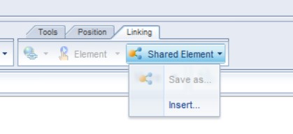
  • Web Intelligence – Shared Elements

This is the starting point for something that I have always desired to see in Web Intelligence. For many years I have wanted a way to define a central report variable repository. While it’s not quite implemented the way I desired, within the shared elements feature, the end results is much the same. Hopefully they will take this a step further in the future but I can live with shared elements for now.

With that said, developers now have the option to publish report elements to a central located platform public folder. They can also refresh or re-sync these elements using the new shared elements panel within Webi. While this might not seem like an earth shattering enhancement, let’s take a moment to discuss how this works and one way we can use it to our advantage.

Take for example, a report table. Within that report table I have assigned a few key dimensions and measures. I have also assigned 5 report variables. These variables contain advanced calculations that are critical to the organization. When I publish this table to a shared elements folder, the table, dimensions, measures and variables are all published. That’s right, the variables are published too. Later on I can import this shared element into another report and all of the dimensions, measures and variables are also imported with the table. One important functionality note is that Web Intelligence will add a new query to support the shared elements containing universe objects. It does not add the required dimensions and measures to any existing query. This might complicate matters if you are only attempting to retrieve the variables. However, you can manually update your variable to support existing queries.

Shared_elements

If you have not had the epiphany yet, let me help you out. As a best practice, we strive to maintain critical business logic in a central repository. This is one of many ways that we can achieve a single version of the truth. For the first time, we now have the ability to store Web Intelligence elements (including variables) in a central repository. Arguably, I still think it would be better to store variables within the Universe. However, shared elements are a good start. Assuming that developers can communicate and coordinate the use of shared elements, reports can now be increasingly more consistent throughout the organization.

I don’t want to underscore the other great benefits of shared elements. Variables are not the only benefit. Outside of variable, this is also an exceptional way for organization to implement a central repository of analytics. This means user can quickly import frequently utilized logos, charts and visualizations into their reports. Because the elements have all their constituent dependencies included, user will find this as an excellent way to simplify their self-service needs. I find it most fascinating in terms of charts or visual analytics. For the casual user they don’t need to focus on defining the queries, formats, and elements of the chart. They can simply import someone else’s work.

  • Web Intelligence – Parallel Data Provider Refresh

I was quite pleasantly surprised that this enhancement was delivered in 4.2. In the past, Web Intelligence would execute each query defined in a report in serial. If there were four queries and each required 20 seconds to execute, the user would have to wait 4 x 20 seconds or 80 seconds for the results. When queries are executed in parallel, users only have to wait for the longest running query to complete. In my previous example, that means that report will refresh in 20 seconds not 80 seconds. Keep in mind that you can disabled this feature. This is something you might have to do if your database can not handle the extra concurrent workload. You can also increase or decrease the number of parallel queries to optimize your environment as needed.

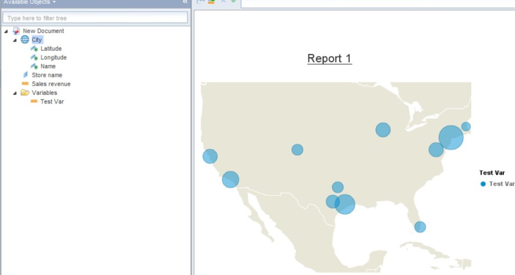
  • Web Intelligence – Geo Maps

Maps in Web Intelligence? Yes really, maps in Web Intelligence are no longer reserved for the mobile application. You can now create or view them in Web Intelligence desktop, browser or mobile. The feature also include a geo encoder engine. This engine allows you to geocode any city, state, country dimension within your existing dataset. Simply right click a dimension in the “Available Objects” panel to “Edit as Geography” A wizard will appear to help you geo encode the object. Note that the engine runs within an adaptive processing server and the feature will not work unless this service is running. I found this true even when using the desktop version of Web Intelligence.

geo_maps

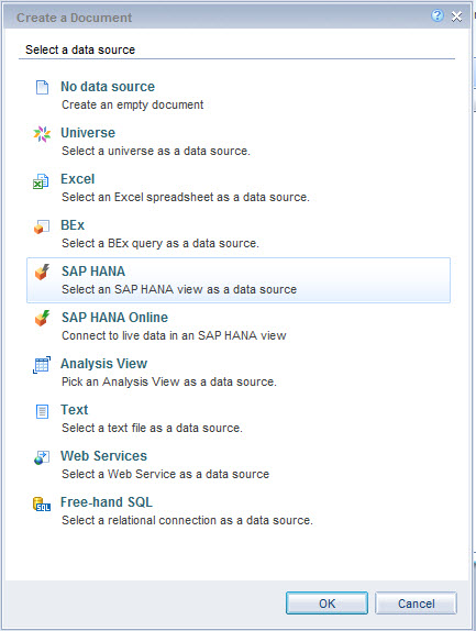
  • Web Intelligence – Direct access to HANA views.

For those that did not like the idea of creating a Universe for each SAP HANA information view, 4.2 now allows the report developer to directly access a SAP HANA information view without the need to first create a universe. From what I can decipher, this option simply generates a universe on the fly.

However, it appears that metadata matters. The naming of objects is based on the label column names defined within SAP HANA. If you don’t have the label columns nicely defined, your available objects panel will look quite disorganized. In addition, objects are not organized into folders based on the attribute view or other shared object semantics. With that said, there is an option to organize dimension objects based on hierarchies defined in the HANA semantics. However, measures seem to be absent from this view in Web Intelligence (relational connections) which makes me scratch my head a little. Overall, I think it’s a great option but still just an option. If you want complete control over the semantics or how they will be presented within Web Intelligence, you still need to define a Universe.

Webi

  • Web Intelligence – SAP HANA Online

Let me start by saying this, “this is not the same as direct access to HANA views”. While the workflow might appear to be similar, there is a profound difference in how the data is processed in SAP HANA online. For starters, the core data in this mode remains on HANA. Only the results of your visualization or table are actually transferred. In addition, report side filters appear to get pushed to SAP HANA. In other modes of connecting to HANA, only query level filters are pushed down. In summary, this option provides a self-service centered option that pushes many of the Web Intelligence data process features down to HANA.

As I discovered, there are some disadvantages to this option as well. Because we are not using the Web Intelligence data provider (micro cube) to store the data, calculation context functions are not supported. The same is true of any function that leverages the very mature and capable Web Intelligence reporting engine.  Also, the semantics are once again an issue. For some reasons, the HANA team and Web Intelligence team can’t work together to properly display the Information view semantics in the available objects panel. Ironically, the semantics functionality was actually better in the 4.2 SP1 version than in the GA 4.2 SP2 release. In 4.1 SP1, the objects would be organized by attribute view (Same for Star Join calculation views). Webi would generate a folder for each attribute view and organize each column into the parent folder. In 4.2 SP2 we are back to a flat list of objects. In your model has a lot of objects, it will be hard to find them without searching. I’m not sure what’s going on with this, but they need to make improvements. For large models, there is no reason to present a flat list of objects.

Regardless of these few in number disadvantages, this is a really great feature. It truly has more advantages than disadvantages. User gain many of the formatting advantages of Webi while also leveraging the data scalability features of SAP HANA. As an added bonus, the report side filters and many other operations are pushed down to SAP HANA which makes reporting simple. User do not have to focus so intently on optimizing performance with prompts and input parameters.

  • IDT – Linked Universes

We can finally link universes in IDT. UDT (Universe Design Tool) had this capability for many years. I am not sure why it was not included with IDT (Information Design Tool) from the beginning. That’s all I have to say about that…

  • IDT – Authored BW BEx Universes

As proof that users know best, SAP relented and we can now define a Universe against a BEx query. No Java Connector or Data Federator required. This option uses the BICS Connection which offers the best performance. To me this all boils down to the need for better semantics integration. The same is also true of SAP HANA models. Having the ability to define a UNX universe on BEX queries has a lot to do with the presentation and organization of objects. For some strange reason users really care about the visual aspects of BI tools (and yes that last statement was sarcasm).

There are also option to change how measures are delegated. Measure that do not require delegation can be set to SUM aggregation. Fewer and fewer #ToRefresh# warnings I hope…

  • Platform – Recycle Bin

One of the more frustrating aspects of the platform over the last few decades was the inability to easily recover accidentally deleted items. In the past, such a recovery required 3rd party software or a side car restore of the environment. If you didn’t have 3rd party software or a backup, that deleted object was gone forever.

Recycle

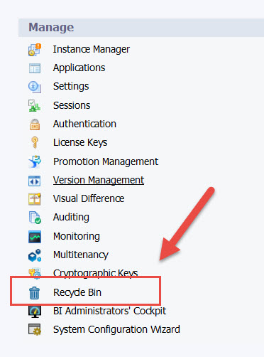
Once enabled, the Recycle Bin will allow administrators to recover deleted objects for a configurable amount of time. For example, we can choose to hold on to objects for 60 days. Only public folder content is support as well and user’s cannot recover objects without administrator help. However, this is a great first step and a feature that has been needed for over a decade.

  • Platform – LCMBIAR files

Well it only took a few years but we can finally selectively import objects contained in an LCMBIAR file within the promotion management web application.  Ironically I really wanted this functionality a few years ago to help with backups. Specifically public folder backup to aid users that accidentally deleted objects.  Now that SAP designed the recycle bin, there is less of a need for this solution.

Prior to the latest enhancement, you had to import all objects in an LCMBIAR file. If I only wanted 1 of 8000 objects in the file, I had to import it into a dedicated temporary environment and then promote just the needed objects into the final environment.

  • Platform – Split Installer

Using the installation command line, administrators can now prepare the system for installation without down time. It does this by performing all of the binary caching and some of the SQL lite installation database operations before it invokes the section of the install that require down time. Running setup.exe –cache will invoke the caching portions of the install. When ready to complete the install, running setup.exe –resume_after_cache will complete the insulation. In theory, the later portion of the installation step reduces the down time by eliminating the dependency between the two major installation and upgrade tasks.

In large clustered environment this is a great addition. In all types of environments this is a great enhancement. Previously the system down time was subjected to the long and tedious process of caching deployment units.

  • Platform – New License Keys

After you upgrade to 4.2 SP2, you will need to obtain a new license keys. The keys that once worked for 4.0 and 4.1 will not work after upgrading to 4.2 SP2. The graphical installer will also let you know this. Be prepared to logon to service market place and request new keys.

More Information and links

I only mentioned what I thought to be the most interesting new features. However there are several other features including in 4.2 SP2. The following links contain more information about the new features in SAP BOBJ 4.2 SP2.

New Publication – SAP HANA High Availability and Disaster Recovery Essentials


Checkout the latest SAP Insider book

http://store.sapinsider.wispubs.com/products/SAP-HANA-High-Availabilty-and-Disaster-Recovery-Essentials.html

SAP HANA provides speedy access to your data, but only if everything is running smoothly. This anthology, a collection of articles recently published in SAP Professional Journal, contains tips and best practices on how to ensure that your data is highly available despite any system mishap or disaster that may occur.

For example, Dr. Bjarne Berg shows you how to create a standard operating procedure (SOP) checklist that contains the daily operations, weekly jobs, and period upgrades and patches needed to keep your SAP HANA system up and running. Jonathan Haun calls on his extensive experience with SAP HANA to give you an overview of its disaster recovery (DR) and high availability (HA) options. In a second article, he provides advice on the backup and restore process. And in his third piece, he explains how you can protect your data using SAP System Replication. Security expert Kehinde Eseyin lists 25 best practices for preventing data loss, while Rahul Urs gives an in-depth look at SAP HANA’s security functions. Ned Falk follows up on one of Kehinde’s tips, explaining how to set up the system usage type feature. The feature lets you know if you are in a production versus a test system, preventing you from inadvertently causing a database issue. Irene Hopf gives an overview of best practices in a data center to ensure business continuity.

Finally, we offer you two bonus articles that give you a taste of other SAP HANA topics covered in SAP Professional Journal. These are written by Christian Savelli, Dr. Berg, and Michael Vavlitis.

Table of Contents

Protect Your SAP HANA Investment with HA and DR Options…………………… 3
by Jonathan Haun, Consulting Manager, Business Intelligence, Decision First Technologies
Implementing an SAP HANA system involves more than just selecting a standalone server. Organizations must also consider the different options available in terms of high availability (HA) and disaster recovery (DR). Depending on the organization’s service-level requirements, multiple servers, storage devices, backup devices, and network devices might be required. This article gives an overview of the different ways organizations can achieve SAP HANA HA and DR. Equipped with this information, you can develop the right SAP HANA architecture and business continuity strategy more easily.

Mastering the SAP HANA Backup and Restore Process………………………….11
by Jonathan Haun, Consulting Manager, Business Intelligence, Decision First Technologies
When organizations implement SAP HANA, they need to devise a strategy to protect the data that the system manages in memory. Depending on your SAP HANA use case, failure to protect this data can lead to significant monetary or productivity losses. One way to protect the data is through the implementation of a backup and restore strategy.This article helps to fortify your general knowledge of the SAP HANA backup and restore process. It also discusses a few key questions that should be asked when devising a backup strategy for SAP HANA.

Prevent Data Disaster in Your SAP HANA System Landscape with Effective Backup and Restore Strategies …………………28
by Kehinde Eseyin, Senior SAP GRC Consultant, Turnkey Consulting Ltd.
Become acquainted with concepts, best practices, optimal settings, tools, and recommendations that are invaluable for SAP HANA database backup and restore operations.

SAP HANA’s System Usage Type: Use This Simple Setting to Prevent Major Mistakes in Your Production System …………..50
by Ned Falk, Senior Education Consultant, SAP
Learn the steps needed to configure the SAP HANA Support Package 8 system usage type feature to enable warnings when the SAP system thinks you’re doing things you should not be doing in your SAP HANA production system.

No, Your SAP HANA-Based Data Center Is Not as Simple as a Toaster………56
by Irene Hopf, Global Thought Leader for SAP Solutions, Lenovo
Learn how to set up business continuity in SAP HANA with high availability, disaster recovery, and backup/restore concepts. This overview shows the challenges of managing SAP HANA-based applications in the data center.

How SAP HANA System Replication Protects Your Data…………………….62
by Jonathan Haun, Consulting Manager, Business Intelligence, Decision First Technologies
When organizations implement SAP HANA, they need to devise a strategy to protect the data that the system manages in memory. Depending on your SAP HANA use case,failure to protect this data can lead to significant monetary or productivity losses. One way to protect the in-memory data is through the implementation of SAP HANA System Replication. SAP HANA System Replication is a solution provided by SAP that works with all certified SAP HANA appliance models. It also works with Tailored Datacenter Integration (TDI) configurations if you build your own system using TDI rules.

Tips on How to Secure and Control SAP HANA …………………………….75
by Rahul Urs, GRC Solutions Architect, itelligence, Inc.
Learn how to implement security and controls in SAP HANA and understand key areas of SAP HANA security, such as user management, security configuration, security and controls for SAP HANA, security flaws, and common oversights.

Avoid SAP HANA System Surprises with a Standard Operating Procedure Checklist…………..81
by Dr. Bjarne Berg, VP SAP Business Intelligence, COMERIT, Inc., and Professor at SAP University Alliance at Lenoir Rhyne University
Keep your SAP HANA system up and running with these preventive measures and tips for regular monitoring of system activities.

Bonus Article: Complement Warm Data Management in SAP HANA via Dynamic Tiering………..105
by Christian Savelli, Senior Manager, COMERIT, Inc.
This bonus article describes the Dynamic Tiering option available starting with SAP HANA Support Package 9, which enables a more effective multi-temperature data strategy. It offers management of warm data content via the extended table concept, representing a major enhancement from the loading/unloading feature currently available. The main benefit offered is more control over the allocation of SAP HANA main memory and corresponding mitigation of risks associated to memory bottlenecks.

Bonus Article: SAP HANA Performance Monitoring Using Design Studio……………113
by Dr. Bjarne Berg,VP SAP Businesss Intelligence, COMERIT, Inc., and Professor at SAP University Alliance at Lenoir Rhyne University,and Michael Vavlitis, SAP BI Associate and Training Coordinator, COMERIT, Inc.
This article is a sampling of the content for system administrators you can find in SAP Professional Journal. Learn the details around the process of developing and implementing SAP HANA performance monitoring using an application built by SAP BusinessObjects Design Studio. Active performance monitoring is a vital measure formaintaining the stability of an SAP HANA system, and Design Studio offers the ideal capabilities to track the most important SAP HANA performance indicators.

My favorite “What’s New” feature of SAP BusinessObjects 4.1 SP5


This posting is a little “late to the press” but I thought I would follow tradition and post a what’s new for SAP BusinessObjects 4.1 SP5. Most of the important details are listed in the What’s New Guide on help.sap.com. However I did find that a major enhancement had been implemented in the SAP BusinessObjects Explorer 4.1 SP5 plugin. From what I can tell, this enhancement was not listed in the “What’s New” guide. I was actually notified of the enhancement through ideas.sap.com.

So what is the major enhancement? Drumroll please……you now have a few formatting options when defining calculated measures within an SAP Explorer Information Space.

You can now format calculated measures defined in your SAP Explorer Information Space.

You can now format calculated measures defined in your SAP Explorer Information Space.

Explorer Formatting Numbers

This includes the ability to define the number of decimal places and Currency Symbol

Previously you only had formatting options when your information space was based on a Universe. The Information Space would inherit the formats defined on the measures derived directly from the Universe. However, calculated measures (those defined in the information space) had no formatting options. This was of particular importance when BWA or SAP HANA were the prescribed data source (IE… No Universe was utilized).

One of the most common KPI’s used by business is % Change. To calculate percent change in Explorer, you have to first define its numerator and denominator as separate measures in the source. Using a calculated measure, you could then perform the division to produce a raw change ratio number. Without the ability to format the number in the presentation layer, business users had to view the measure in its raw decimal format. For example, they would see .3354 in an Explorer Chart or table. What they really desired was the ability to view the measure formated as 33.5%. While this might seem like a trivial feature, I can attest that multiple customers found this to be a huge issue. Business user want to see the KPI in “%” format. “That is how it has always appeared in previous tools”. Fortunately SAP finally added the feature in SAP BusinessObjects Explorer 4.1 SP5.

There are a few other changes in SP5 as well. You can now define Web Intelligence customizations on the User Group and Repository folder level. This means that you can pick and choose the Web Intelligence UI buttons that are visible based on group membership or folder location.

Unfortunately it is now impossible to figure out the forward fit plan for 4.1 SP5. SAP Note 2103001 tries to explain the new forward fit process but your guess is as good as mine. Maybe this posting will get some feedback explaining how to determine the forward fit for a patch or support pack?


Why do join types matter in a SAP HANA information view


What are we joining?

When you design an SAP HANA information view, we must also define joins between tables or attribute views. These joins can be configured in the foundation of attribute views and analytic views. They can also logically occur in analytic and calculation views.

Why do joins matter?

In some cases, joining tables can be an expensive process in the SAP HANA engines. This is especially true when the cardinality between tables is very high. For example, an order header table with 20 million rows is joined to an order line detail table with 100 million rows. Excessive joining in the model is also something that can lead to performance issues. Excessive joining is something that occurs often when we are attempting to denormalized OLTP data using SAP HANA’s information views.

What is the solution to work around join cost?

Join pruning is a process where SAP HANA eliminates both tables and joins from its execution plan based how the joins are defined in the information view and how data is queried from the information view.

For example, let’s assume that we have a customer table or attribute view configured with a left outer join to a sales transaction table in our analytic view.  If we query the information view and only select a SUM(SALES_AMOUNT) with no GROUP BY or WHERE clause, then the execution plan might skip the join process between the customer table and the sales transaction table. However, if we execute SELECT CUSTOMER_NAME, SUM(SALES_AMOUNT) then the join between the customer table and sales transaction will be required regardless of the join type used.

The process is subjective and related to how the joins are configured in our information view. It is also subjective to how the information view is queried. If every query we execute selects all attribute and measures, then join pruning would never be invoked. Fortunately, in the real world, this is not typically the case. Most queries only select a subset of data from the information view. For this reasons, we should try to design our information views to take advantage of join pruning.

What join options do I have?

There are five main types of joins to look at in this context. Inner Joins, Referential Joins, Left Outer, Right Outer and Text Joins. Below is an outline on how SAP HANA handles each join type.

INNER JOIN

Inner Joins are always evaluated in the model. No join pruning occurs because an inner join effectively tells the SAP HANA engine to always join no matter what query is executed. Records are only returned when a matching value is found in both tables. Overall they are one of the most expensive join types that can be defined in an information view. They also have the potential to remove records from the results assuming that referential integrity is poorly maintained in the source tables.

REFERENTIAL JOIN

For all intents and purposes, the referential join acts like an inner join. However, under specific circumstances, the referential join will be pruned from the execution of the information view. Assuming that there are no filters defined in an attribute view’s foundation, the SAP HANA engines will likely prune the join from the execution plan of the analytic view. This assumes that no columns are queried within the same attribute view.  However, if a column from the attribute view is included in a query, this join will act as an inner join.

Let me reiterate the exception to the pruning rule one more time. If filters are defined in the attribute view, the join will be included and enforced as an inner join even if no attribute view columns are selected. This means that records are only returned when a match is found in both the attribute view and analytic view foundation table. It also means that referential joins are not always pruned from the information view execution plan. Pay close attention to this exception because referential joins can be just as expensive as inner joins.

When a referential join is pruned we have to make sure that the referential integrity between tables is sound. If it is not, we might get varying results based on the columns selected in our queries. For example, a transaction might not have a shipped date defined. When we query for transactions with a shipped date, this transaction would be excluded. When we exclude any shipped date attributes from our query, the transaction would magically appear again because of join pruning. Based on experience, this can confuse the heck out of an end user… or a developer 🙂

LEFT OUTER

Based on several query scenarios that I tested, the left outer join is always pruned from the execution plan assuming that no columns are selected from an attribute view defined within the model. Left outer joins are often defined in instances where the analytic view foundation table is known to have no matching record within an attribute view. By design, they prevent the model from excluding transactions. This is because it will ensure that all possible transactions are returned, even if we are missing master data. Overall I would say that the left outer join has the potential to be the best performing join within our information view definition.

However, we have to make sure that it makes sense before we arbitrarily set up our models with left outer joins. We sometime need the inner join to help exclude records. For example, let’s assume that we have a date attribute view joined to a data column in our analytic view foundation table. Using an inner join we can exclude any transaction that has no defined date. There are other instances where we might find phantom transactions in our aggregates with a left outer join. For example, a transaction that has no customer, date or product. In those cases, something was likely only partially deleted from the system. Therefore, referential integrity issues can create problems.If you recall a similar issue can happen with referential joins. However, with left outer joins we will always return the transaction.

RIGHT OUTER

The right outer join is used in instances where all attribute view values need to be returned even if they have no matching transactions.  For example, I need a complete list of all customers even if they have never been issued an invoice. This would be helpful if the query were targeting both existing and potential customers.

Keep in mind that a mismatched transaction will be excluded from any analytic view’s aggregates. Based on my testing, a right outer join is always performed in the execution of the model. I was not able to devise a single scenario where the join was pruned from the execution of the model. With this in mind, it will have a high cost when used in the information view definition.

TEXT JOIN

This is effectively an inner join setup specifically to work with the SPRAS field found in SAP BusinessSuite tables. Based on my brief testing, it is always executed and never pruned from the model.

What’s new in SAP BusinessObjects 4.1 SP4


A few weeks ago SAP released SAP BusinessObjects 4.1 Support Pack 4 (SP4). This package introduced a few new features which are listed in the “What’s New guide”. It also introduced compatibility or support for  s few new items. There is not much to talk about so ill keep in brief.

New Feature (Highlights)

  1. The translation manager now supports Analysis for OLAP documents.
  2. A few Web Intelligence charting enhancements
  3. You can now schedule BEx based Web Intelligence reports where the BEx query contains dynamic variables.

Supported Platforms (Highlights)

  1. Support for Microsoft SQL 2014
  2. Support for Oracle 12c
  3. Support for SAP HANA SPS 08
  4. Official support for Adobe Flash Player 12

Links

The Official “What’s New” guide from SAP

SAP BusinessObjects Enterprise PAM (4.1 SP4)

Forward Fit Document

Forward Fit information

Contains the fixes found in the following releases

4.1 SP 3.1
4.1 SP 2.3
4.1 SP 1.7
4.0 SP 9.1
4.0 SP 8.5
4.0 SP 7.9
4.0 SP 6.12

An agile and relevant BI foundation built on SAP HANA


If you are active in the SAP ecosphere and you have somehow managed to never see or hear anything about SAP HANA, I can only conclude the following. You obviously live under a rock in the deepest darkest forest on a planet in a distant galaxy where SAP has yet to establish a sales territory. All joking aside, it is very unlikely that SAP HANA has not been at the forefront of most SAP related discussion in recent years. For those that know about SAP HANA, I would bet that your first thought is always related to one word. That word is “fast”. SAP HANA is an in-memory, columnar store and massively parallel analytical data processing engine. For the average business intelligence (BI) consumer this conglomeration of adjectives and technical terms mean one thing; it’s fast.  If we accept that SAP HANA is fast, we have to ask ourselves what do I gain with speed? We then have to ask is speed alone a primary reason to purchase SAP HANA?

What do I gain with speed?

Below I will list a few of the more obvious reasons that speed maters. There are other reasons not listed but this will help start the thinking process.

Productivity

It is very easy to argue that we are more productive when we spend less time waiting for software to respond. In the golden oldie days of BI, we would often endure a query that required 30 + minutes to execute. That was 30 minutes of time we had to do something else. I like to call these queries the “coffee break queries”. This is because we often use this time to go get coffee.  If we can reduce these queries to seconds with SAP HANA, users will be more likely to stay engaged and remain productive.

Depth

Speaking of 30 minute queries, can you imagine how unwilling a consumer would be to explore their data if every perspective change required a 30 minute wait time? My experience is that users quickly loose interest in exploring their data when the software is too slow to respond. If we could reduce these queries to seconds, users will be more likely to not only be productive but to also dig a little deeper into their data. Think of SAP BusinessObjects Explorer running on SAP HANA. Users can take a billion row dataset and explore it from multiple perspectives. Because of speed, we can now gain better depth into our data.

Data Loading

When we think of speed, we often focus on the consumer’s experience. However, daily IT processes can also be accelerated with SAP HANA due to the increased data loading capabilities. If your legacy data load process required 14+ hours, most SAP HANA solutions will likely reduce that by more than 50%. This gives IT departments more time to recover from data load failures or to extend the scope of the data set. It also provides the data consumer with a greater chance that their data will be available the next day.

Competitive Edge

As a general rule, if we can outthink and respond faster to a changing economic climate, we often gain a competitive edge over our competition. In some ways, SAP HANA can helps us do that. SAP HANA cannot think for us but it can help us discover trends, identify changes, understand our successes, identify our failures and accelerate other areas of our business. Most organizations can already do all of these things effectively with their current BI environments. However, imagine how much better it will be when it happens faster with larger and more complex datasets.

Customer satisfaction

Another competitive advantage for organizations is their ability to service their customers. Speed can help an organization better understand their customer by instantly analyzing past history and predicting future needs. This can be done quickly and on the fly when we have speed. With that advantage we can start embedding sophisticated analytics in our frontend applications. Take for example a call center. If we enter the customer’s details into a system, we can then have a series of analytics pop-up that help us understand the customer relationship to our organization. We can also suggest products and services they might be interested in based on these analytics. This is all achievable because of speed.

Is speed alone the main reason for purchasing SAP HANA?

Query and processing speeds alone are not the only reasons to purchase SAP HANA. There is more to SAP HANA than just speed. Speed allows an organization to achieve technical wonders but behind the speed is a process. There must be a process for obtaining data that is consistent, repeatable and reliable. For years we have known this as the Enterprise Information Management (EIM) process. Using processes and tools, organizations can obtain data, model it into usable structures and then load it into a database for querying.  The process also helps other initiatives such as data governance, data quality and a “single version of the truth”.

The down side to the processes is that obtaining new data is often seen as slow and cumbersome by the data consumers. They often have to wait weeks or months before data is available to them. This happens for a variety of reasons. IT resources often have to first find the data, develop a processes to capture it on a recurring basis and then deal with any gaps or inconsistencies. That is not necessarily a problem that can be overcome with any level of speed or technology. The hope is that these complexities subside after a strong data governance program is instituted. One where the organization begins to manage data as an asset as opposed to a byproduct. In short, only processes and management can fix part of the EIM problem.

However, there is another side to EIM that has evolved around the needs of the data consumer. There is more to data than just storing it in a Kimball / Inman star schema of tables. Users have to be able to construct or access queries that can answer relevant business questions. If we solve these problem with the EIM process alone, we often end up with extra aggregate tables, custom fact tables or a variety of different tables formulated to help query processing. Unfortunately, these extra tables add more and more time to the recurring data update process. As the processing time and complexity of managing these processes increases, the data consumer becomes more and more impatient. With the traditional RDBMS, these extra tables are also sometimes required because of the inefficiencies of the row store and spinning disk. With SAP HANA, we can begin rethinking this strategy on all fronts. SAP HANA’s speed helps us reshape this strategy but there is more to this story than speed.

Let’s not forget the SAP HANA also has something special built-in to its data platform. SAP HANA has multidimensional models built directly into the database. By name they are called attribute views, analytic views and calculation views. In a generic since, they act as a semantic layer. They are often called information views or information models. They act as a layer that exists between the database tables and the data consumers. They provide easy, consistent and controlled access to the data.

In a traditional BI landscape, this semantic layer is typically separated from the RDBMS. However, with SAP HANA it is directly integrated. In some BI products, this layer acts as a separate data store. Take for example the traditional OLAP cube. OLAP cubes, using MOLAP storage, not only store the metadata but they also store the actual data. They act like a supercharged BI database but they require extra time to load. Then there are technologies such as the SAP BusinessObjects universe. It takes a ROLAP approach where data is kept in the database and only metadata is stored in the semantic layer.  This cuts down on the data load times but the semantic layer interface is typically proprietary. This means its not universally possible for most BI tools to access the semantic layer. In most cases the same is true of the OLAP cube because not every BI tool has an interface to its data. The MOLAP and ROLAP methodologies both have multiple benefits which are beyond the scope of this posting. However, one thing is clear with the legacy semantic layer. It has traditionally been separated from the RDBMS and it often only works with a limited set of BI tools.

SAP HANA is different, though. To understand how it is different lets answer a few questions. One, how does SAP HANA help the overall EIM process? Two, how do we leverage the SAP HANA multidimensional information models to aid consumers?

SAP HANA helps the overall EIM process by eliminating the need to create special use tables and pre-aggregate tables. With SAP HANA, these tables can be converted into logical information views and accessed with SQL. By eliminating these persistent tables, we are reducing the time required to execute the recurring data update process.  These same information views also help IT to make changes faster. By reducing the number of physical tables in the model, IT developers are able to make changes without the need to also update data found in downstream tables.  The basic idea is that logical information views are more agile than maintaining the equivalent physical table.

If we assume that agility is an important benefit of SAP HANA, we must also consider relevancy. Getting content to the consumer quickly is part of the battle. We also have to make sure that the content is relevant. This means that we need to make sure that the content helps the consumer answer relevant questions. This is also an area where the information view helps the consumer. Developers can create custom logical models that contain relevant data attributes and measures.  Because they are embedded into the RDBMS and centrally located, these views can also be accessed by any tool that supports the SAP HANA ODBC, JDBC or MDX drivers. This helps an organization to maintain a single version of the truth while simultaneously providing an agile and relevant foundation for the consumption of data.

SAP HANA Foundation

The above figure helps to illustrate this benefit. Starting at the bottom we wrap the entire process into the Data Quality and Data Governance umbrella. This means that these processes govern everything we do in SAP HANA. We then focus on how the data gets into SAP HANA tables. This can be a daily batch Extract Translate Load (ETL) processes with SAP Data Services or a daily delta load using the BW extractors into a BW on HANA instance.

We also have to look at the Extract Load Translate (ELT) processes. This includes instances were SAP Landscape Transform (SLT), SAP Replication Services or SAP Event Stream Processor (ESP) is used to provision data, in real-time, into SAP HANA. As an added bonus we can also add BI solutions built into SAP Business Suite on HANA in this area.

The provisioning solution that is used at this layer all depends on the data consumer’s requirements and the organization’s needs. However, the goal at the data provisioning layer is to minimize the amount of data duplication and eliminate the need for subsequent processing into additional tables. Data should be stored at its lowest level of granularity in either a normalized or denormalized fashion. Ideally it is only stored in a single location that can be reused in any information model.  For example, this means we can focus on developing the base FACT and DIMENSION tables, DSOs or replicating normalized ECC tables. Anything that is required above this layer should be logical. This is not to say that we can facilitate all needs with logical models, but it should be the preferred methodology to facilitate an agile foundation.

Above the physical table layer we also have what I am calling the “Business View” layer. This is the layer where we achieve two goals. One, we try to do the bulk of specialized transformations and calculations at this layer. The SAP HANA information views are logical and do not require the movement of data. This makes them agile when changes are required. Second, we try to construct views that facilitate the needs of the data consumer. By maintaining relevant views, data consumers will be satisfied productive decision makers.

At the top of the diagram we have the SAP BusinessObjects BI tools. Ideally we would use SAP BusinessObjects but other 3rd party tools can also be considered. Regardless of the type of tool, SAP HANA information views should be the primary point of access. This is because they should contain all of the relevant transformations, security and calculations.  Again, they are centralized which helps foster a single version of the truth throughout the organization.

In summary, beyond speed there are two other fundamental benefits of SAP HANA. Agility and Relevancy are also benefits of SAP HANA. Regardless of the SAP HANA solution we choose, agility and relevancy can be leveraged. They might be implemented in slightly different ways but the goal should remain the same. As an added benefit we can also expect great performance (in other words “Speed” helps too).

Click here to watch a video where I explain this in more detail

SAP HANA and Intel’s Ivy Bridge v2


Many hardware vendors are on the verge or have already released their new certified SAP HANA servers based on the Intel Ivy Bridge v2 CPU and related chip sets. So what does this actually mean to the consumer?

  1. A faster RAM chip means faster query response time. The Ivy Bridge v2 CPU support DIMMS based on the DDR3-1066, 1333 or 1600 MHz architecture. The previous generation of servers only supported DDR3 memory clock speeds of  800, 978, 1066, 1333 or 1066. Faster clock speeds mean faster seek times. The net result is a faster SAP HANA system.
  2. A faster CPU clock also means faster query response times. The certified SAP HANA systems running the Ivy Bridge v2 CPU support clock speeds of 2.8 GHz with turbo speeds of 3.4 GHz. The previous generation of E7 CPU operated at 2.4 GHz with turbo speeds of 2.8 GHz. A faster clock means fewer wait cycles and a faster SAP HANA system.
  3. The Ivy Bridge v2 CPU supports 15 cores per CPU socket. This allows SAP HANA to perform more parallel calculations which results in faster speeds and greater workloads. There are more benefits as well:
    1. This allows hardware vendors to supply customers with a 4 sockets (60 core) server that supports 1TB of RAM. Unless something recently changed, SAP has always maintained that the ratio between RAM and CPU core needs to be around 16GB per Core for analytical solutions. The previous generation of 10 core CPUs could only achieve his with an 8 socket motherboard. Because Ivy Bridge V2 supports 15 cores per socket, vendors can now operate 4 socket SAP HANA systems that host 1 TB of RAM. In general this will help reduce the cost of the 1TB server. 8 socket chassis and motherboards are generally very expensive. A 4 socket alternative will likely be less expensive.
    2. For S0H (Suite on SAP HANA) the ratio is different. In general 32GB per core is supported. This means that a 4 socket (60 core) server can now host 2TB of RAM. This will also greatly reduce the cost of SAP HANA systems operating SoH.
  4. SAP claims that the overall benchmark yields a 2x increase in speed compared to the 1st generation of certified SAP HANA systems. However, I still think we need verify the performance as vendors try to support 1TB of RAM on the 4 socket architecture. If you think about it, the 1st generation 8 socket systems supported 80 cores. The new 4 socket Ivy Bridge v2 systems support 60 cores. Their is a CPU/RAM ratio difference of 80/60 to 12.8GB/17.1GB (1024 GB / 60 or 80). Perhaps the faster memory clock speeds and other enhancements to Ivy Bridge v2 easily overcome any issues?  I guess we will need to wait until official benchmarks are available before passing judgement.
  5. Some vendors are able to build XS (Extra Small) through XL (Extra Large)  SAP HANA systems on the same server chassis and motherboard platform. This will allow organizations to scale up or add RAM and CPU’s as needed. The previous generation of servers were based on a variety of platforms. Often organizations would have to purchase a new server when they needed to scale up.
  6. The logging partition appears to no longer require super fast PCIx Nand Flash cards? The first generation of SAP HANA servers were all equipped with Fusion IO cards or RAID 10 SSD arrays. The 2nd generation appears to have relaxed the IOPS requirements. If this is truly the case, the storage cost for SAP HANA servers should also be greatly reduced. The PCIx cards and SSD arrays are very expensive. If SAP HANA can operate its logging mechanism at optimal speeds, on a partition using more cost effective spinning disks, you should expect a less costly SAP HANA server.
    1. Note: SAP HANA stores and accesses date in RAM. The disks only contain redundant information in case of a power failure. The only conceivable downside to a slower logging partition, is a scenario where  bulk loading large chunks of data to SAP HANA is slowed. It can also affect the SAP HANA startup time. When started, SAP HANA takes ROW data from disk and lazy loads COLUMNAR data as needed. If the anything needs to be recreated from the logs at startup, I would assume that a faster disk is better. The new question is, “how much better”?
    2. Note: I have an open question to SAP on why the logging partition no longer requires fast disks. Something must have changed?


SAP Certified Appliance Hardware for SAP HANAhttp://scn.sap.com/docs/DOC-52522

SAP Certified Enterprise Storage Hardware for SAP HANAhttp://scn.sap.com/docs/DOC-48516

HANA PAM (April 2014) SMP link

Intel E7 8990 v2 CPU specifications

Intel E7 4890 V2 CPU specifications